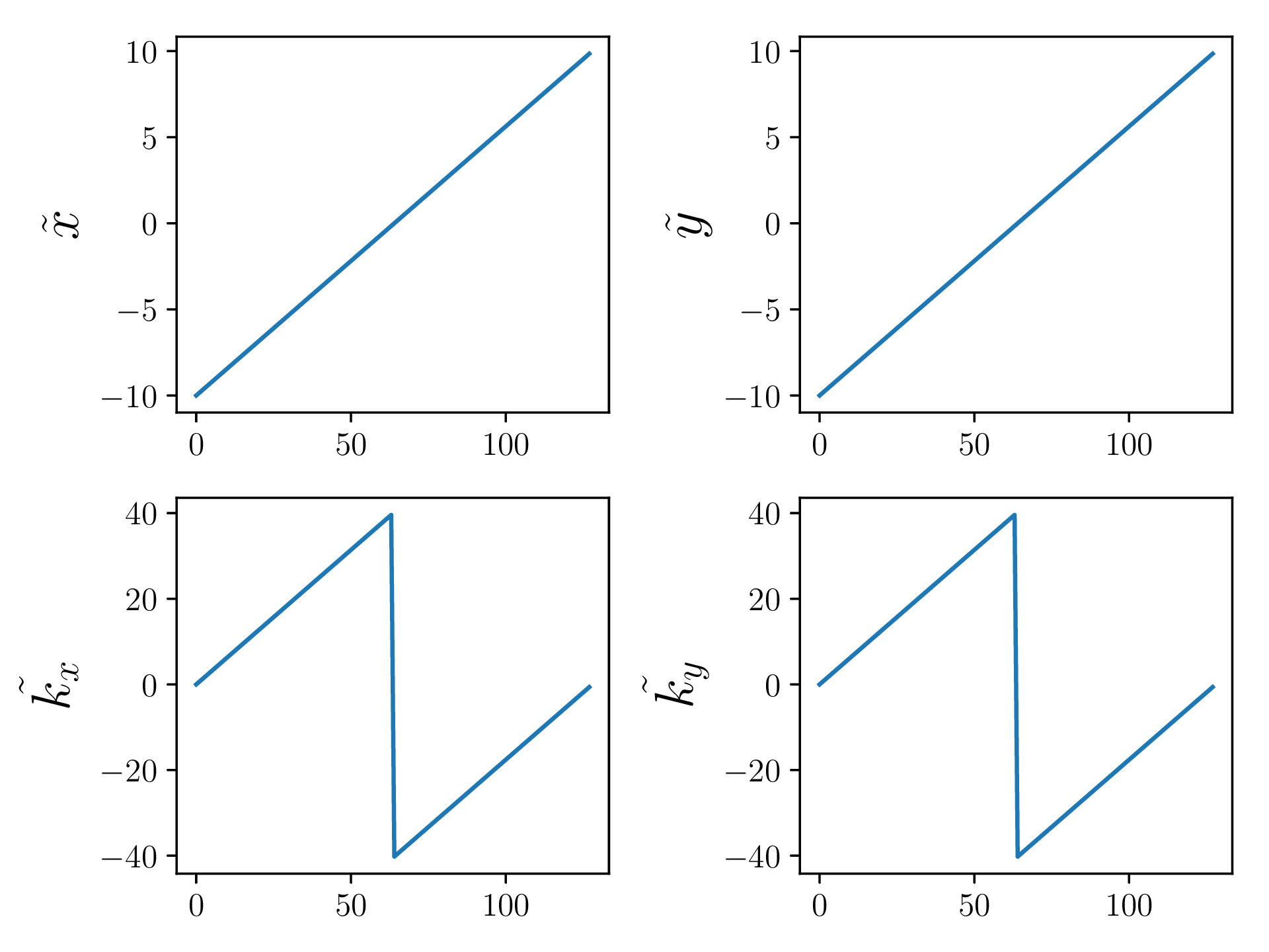
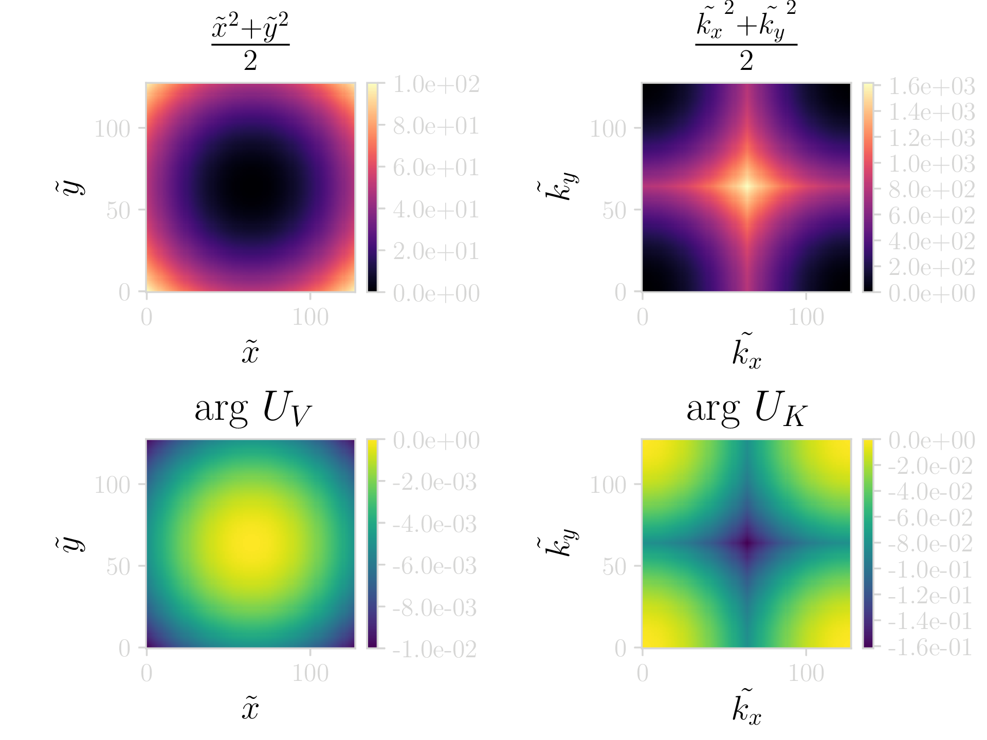
The following article is a work in progress, and will be continually updated over time. I'll issue a RELEASE tag or similar when everything has been finished.

---

Q. How do available FFT routines compare over different libraries and accelerator hardwares?

---

This is something I have wondered for sometime, though it can be difficult for an apples-to-apples comparison. I will consider the above question in relation to the following plan:

Comparing FFT implementations in a pseudospectral solver for linear and nonlinear Schrodinger equation dynamics

To decide on how to proceed, it is instructive to list all (or most) widely known and used implementations.

Standard implementations

[CPU]

• FFTW: http://fftw.org/ and https://github.com/FFTW/fftw3
• MKL-FFT: https://software.intel.com/en-us/articles/the-intel-math-kernel-library-and-its-fast-fourier-transform-routines
• clFFT: https://github.com/clMathLibraries/clFFT
• Eigen FFT (using kissfft backend): http://eigen.tuxfamily.org/index.php?title=EigenFFT
• sFFT: http://groups.csail.mit.edu/netmit/sFFT/code.html
• KFR FFT: https://github.com/kfrlib/fft

[GPU]

• cuFFT: http://docs.nvidia.com/cuda/cufft/index.html
• clFFT: https://github.com/clMathLibraries/clFFT
• fbfft: https://github.com/facebook/fbcuda/tree/master/fbfft and https://arxiv.org/abs/1412.7580

[Cutting edge]

• FPGA FFT (Xilinx and Altera/Intel): https://www.xilinx.com/products/intellectual-property/fft.html and https://www.altera.com/products/intellectual-property/ip/dsp/m-ham-fft.html
• IBM TrueNorth FFT: No link/source found (yet)
• Rigetti pyQuil quantum FFT: http://pyquil.readthedocs.io/en/latest/getting_started.html (currently emulated AFAIK, but will eventually/hopefully run directly on quantum hardware)

Test cases

To ensure sufficient time is spent in the FFT routines I will opt for a 2D transform of an NxN grid, requiring N transforms, a transpose, and another N. The value of N can be scaled to determine sweet spots for all implementations. Granted, memory size will be the determining factor of how large we can go. $N=2^j$ where $j \in \mathbb{Z}, 7 \leq j \leq 11$ is a reasonable range of values to examine that should fit readily on most hardware.

For this, the following test precisions will be instructive:

• $\mathbb{C}2\mathbb{C}$ - 32-bit float (32-bits for each real and imaginary component)

• $\mathbb{C}2\mathbb{C}$ - 64-bit float

• $\mathbb{R}2\mathbb{C}$ - 32-bit float

• $\mathbb{R}2\mathbb{C}$ - 64-bit float

As a sample system to investigate, I will consider the case of a quantum harmonic oscillator (QHO). To investigate dynamics and their resulting accuracy, a known and analytically calculable result is useful. For this, I will opt for a a superposition state of the groundstate along the $xy$ plane, and the first excited state along $x$ with the groundstate along $y$. To put things more formally:

$$\Psi(x,y) = \frac{ \Psi_{00}(x,y) + \Psi_{10}(x,y) }{\sqrt{2}}.$$ To construct the above wavefunction we will assume that the states $\Psi_{00}(x,y)$ and $\Psi_{10}(x,y)$ are outer products of the solutions to the QHO, as given by:

$$\Psi_n(x) = \frac{1}{\sqrt{2^{n}n!}}\left(\frac{m\omega_x}{\pi\hbar}\right)^{\frac{1}{4}}\mathrm{e}^{-\frac{m\omega_x x^2}{2\hbar}}H_n(x),$$ where $$H_n(x)=(-1)^n\mathrm{e}^{x^2}\frac{d^n}{dx^n}\left(\mathrm{e}^{-x^2}\right),$$ are the physicists’ Hermite polynomials. As we are looking for the ground and first excited states ($n=0,1$) we can simplify a lot of the above calculations: $H_0(x)=1$ and $H_0(x)=2x$. Next, we determine the states $\Psi_0(x)$ and $\Psi_1(x)$ as:

$$\begin{eqnarray} \Psi_0(x) = \left(\frac{m\omega_x}{\pi\hbar}\right)^\frac{1}{4}\mathrm{e}^{-\frac{m\omega_x x^2}{2\hbar}},~ \Psi_1(x) = \frac{2x}{\sqrt{2}} \left(\frac{m\omega_x}{\pi\hbar}\right)^{\frac{1}{4}}\mathrm{e}^{-\frac{m\omega_x x^2}{2\hbar}}. \end{eqnarray}$$

Along a single dimension, our system can potentially be in any of the allowed harmonic oscillator states. Therefore, the overall state is given by a tensor product of the state along $x$ and that along $y$. If we assume the dimensionality of the Hilbert space along the $i$-th orthogonal spacial index is finite and given by $d_i$, then the overall system dimensionality (ie the total number of states we can consider) is $d = \displaystyle\prod_{i} d_i$.

Assuming an $n$-dimensional system, where each individual dimension is in the groundstate of the harmonic oscillator, we can define the tensor product state as $$\Psi_n = \Psi_0^{\otimes n} = \Psi_0 \otimes \Psi_0 \cdots \otimes \Psi_0.$$

While the above is fine for a general case, for the purposes of FFTs we have assumed a much simpler system, dealing with combinations of only 2 states. We can then define them as $\Psi_{00}(x,y) = \Psi_{0}(x)\otimes\Psi_{0}(y)$ and $\Psi_{10}(x,y) = \Psi_{1}(x)\otimes\Psi_{0}(y)$. Thus, our final superposition state when filling everything in is given by $$\Psi(x,y) = \left(\frac{m}{\pi\hbar}\right)^{\frac{1}{2}}\left(\omega_x\omega_y\right)^{\frac{1}{4}}\mathrm{e}^{-\frac{m}{2\hbar}\left(\omega_x x^2 + \omega_y y^2\right)}\left(x + \frac{1}{\sqrt{2}}\right).$$

To simplify life, I will assume some of the above quantities are set to unity (i.e. $m=\omega_x = \omega_y = \hbar = 1$). This will not change the dynamics of the simulation, but simplify the equations and the numerical implementation, which can help with improving accuracy. The above equation then becomes $$\Psi(x,y) = \left(\frac{1}{\pi}\right)^{\frac{1}{2}}\mathrm{e}^{-\frac{1}{2}\left( x^2 + y^2 \right)}\left(x + \frac{1}{\sqrt{2}}\right).$$

For a more detailed explanation and approach to the above have a look at Christina Lee’s (albi3ro) blog post on time evolution, which will cover the method I use next.

To be continued

/***

This document will implement the quantum simulation aspects of the code, in as simple a means as possible.

***/
#include<stdio.h>
#include<stdlib.h>
#include<math.h>

#define GRIDSIZE 128
#define GRIDMAX 5
#define PI 3.14159
#define DT 1e-4


//################################################//

struct double2{
    double x;
    double y;
};

//Define the grid on which the simulation will be run.
struct Grid{
    double *x = (double*) malloc(GRIDSIZE*sizeof(double));
    double *y = (double*) malloc(GRIDSIZE*sizeof(double));
    double *xy2 = (double*) malloc(GRIDSIZE*GRIDSIZE*sizeof(double));

    double *kx = (double*) malloc(GRIDSIZE*sizeof(double));
    double *ky = (double*) malloc(GRIDSIZE*sizeof(double));
    double *kxy2 = (double*) malloc(GRIDSIZE*GRIDSIZE*sizeof(double));

    double2 *wfc = (double2*) malloc(GRIDSIZE*GRIDSIZE*sizeof(double2));
    double2 *U_V = (double2*) malloc(GRIDSIZE*GRIDSIZE*sizeof(double2));
    double2 *U_K = (double2*) malloc(GRIDSIZE*GRIDSIZE*sizeof(double2));
};

void setupGrids(Grid *grid){
    double invSqrt2 = 1/sqrt(2);
    //Position space grids
    for (int j=0; j < GRIDSIZE; ++j){
        grid->x[j] = -GRIDMAX + j*(2*GRIDMAX)/((double)GRIDSIZE);
        grid->y[j] = grid->x[j];
    }
    for(int i=0; i < GRIDSIZE; ++i){
        for(int j=0; j < GRIDSIZE; ++j){
            grid->xy2[j+GRIDSIZE*i] = 0.5*(grid->x[i]*grid->x[i]+grid->y[j]*grid->y[j]);
            //Evolution operator in position space
            grid->U_V[j+GRIDSIZE*i].x = cos(-grid->xy2[j+GRIDSIZE*i]*DT);
            grid->U_V[j+GRIDSIZE*i].y = sin(-grid->xy2[j+GRIDSIZE*i]*DT);
            
            //Wavefunction
            grid->wfc[j+GRIDSIZE*i].x = sqrt( 1/PI )*exp( -0.5 * ( grid->x[i]*grid->x[i] + grid->y[j]*grid->y[j] ) ) * ( grid->x[i] + invSqrt2 );
            grid->wfc[j+GRIDSIZE*i].y = 0.;
        }
    }

    //Momentum space grids
    for (int j=0; j < GRIDSIZE; ++j){
        grid->kx[j] = (j<(GRIDSIZE/2)) ? j*2*PI/(GRIDMAX) : -(GRIDSIZE - j)*(2*PI/(GRIDMAX));
        grid->ky[j] = grid->kx[j];
    }
    for(int i=0; i < GRIDSIZE; ++i){
        for(int j=0; j < GRIDSIZE; ++j){
            grid->kxy2[j+GRIDSIZE*i] = 0.5*(grid->kx[i]*grid->kx[i]+grid->ky[j]*grid->ky[j]);

            //Evolution operator in momentum space
            grid->U_K[j+GRIDSIZE*i].x = cos(-grid->kxy2[j+GRIDSIZE*i]*DT);
            grid->U_K[j+GRIDSIZE*i].y = sin(-grid->kxy2[j+GRIDSIZE*i]*DT);
        }
    }
}

//################################################//
int fileIO(Grid *grid){
    //Open files to write
    FILE *f_x = fopen("x", "w");
    FILE *f_y = fopen("y", "w");
    FILE *f_xy2 = fopen("xy2", "w");
    FILE *f_kx = fopen("kx", "w");
    FILE *f_ky = fopen("ky", "w");
    FILE *f_kxy2 = fopen("kxy2", "w");
    FILE *f_U_V = fopen("U_V", "w");
    FILE *f_U_K = fopen("U_K", "w");
    FILE *f_wfc = fopen("wfc", "w");

    //No safety checks because I'm a bad person

    fwrite(grid->x, sizeof(double), GRIDSIZE, f_x);
    fwrite(grid->y, sizeof(double), GRIDSIZE, f_y);
    fwrite(grid->xy2, sizeof(double), GRIDSIZE*GRIDSIZE, f_xy2);
    fwrite(grid->kx, sizeof(double), GRIDSIZE, f_kx);
    fwrite(grid->ky, sizeof(double), GRIDSIZE, f_ky);
    fwrite(grid->kxy2, sizeof(double), GRIDSIZE*GRIDSIZE, f_kxy2);
    fwrite(grid->U_V, sizeof(double2), GRIDSIZE*GRIDSIZE, f_U_V);
    fwrite(grid->U_K, sizeof(double2), GRIDSIZE*GRIDSIZE, f_U_K);
    fwrite(grid->wfc, sizeof(double2), GRIDSIZE*GRIDSIZE, f_wfc);

    //No moar opin

    fclose(f_x); fclose(f_y); fclose(f_xy2); fclose(f_kx);  fclose(f_ky);
    fclose(f_kxy2); fclose(f_U_V); fclose(f_U_K); fclose(f_wfc);
    return 0;
}

//################################################//
int main(){
    Grid grid;
    setupGrids(&grid);
    fileIO(&grid);
}


//################################################//